Defining some terms
This post is all about noise, so lets start with a quick discussion of what noise is. In some contexts noise is defined as whatever part of a signal you don’t care about and would rather ignore. It is a distractor and can obscure the information you want, and is usually what people mean when they’re talking about “signal-to-noise ratios”. In electronics this noise often comes from small random voltage fluctuations in the components themselves, and manifests as a sort of hissing sound, similar to shhhhhh. When evaluating these systems, engineers found that they could model this noise as Additive White Gaussian Noise, which we can break down as:
- Additive
- The composite noisy signal is just the original pure signal with the noise added to it
- White
- The noise has a flat spectrum, which means that all frequencies are present equally. In practice real systems always operate within a finite bandwidth, so to be white the noise just has to be flat within the bandwidth of interest. This term comes from an analogy with light, where light with all wavelengths in equal proportions looks white to human eyes.
- Gaussian
- The values the noise takes follow a gaussian (AKA normal) distribution. This means that values near the mean (usually 0) are more likely than values further away. This part is the focus of this post.
While in most engineering contexts noise is considered unwanted, it turns out to be tremendously useful in many audio synthesis applications. Lots of real-world phenomena have noisy components, from wind to snare drums to raspy violin bowing. Because it’s so common, most computer music and audio processing environments have some mechanism to generate noise, and I spent a little time exploring Pure Data’s [noise~] object.
Spectral Properties
The first thing to do is to check the spectrum to see if PD’s [noise~] object actually gives us white noise. To do this I put together a quick little spectrum viewer called [specplot~]:
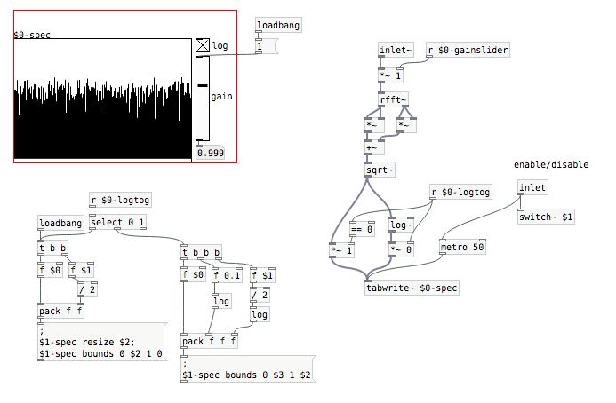
And here’s what the spectrum of [noise~] looks like:
Looks pretty flat to me, which confirms that this is white noise.
Value Distribution
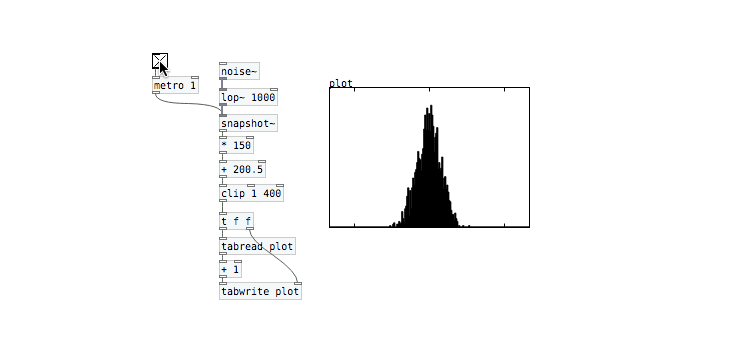
The next question to ask is whether the noise is gaussian-distributed. To check this out we just build a simple match that periodically samples from the noise output and updates a histogram plot. The histogram shows us how often different value ranges show up in the output.
This is definitely not gaussian, but looks more like a uniform distribution. We see that values anywhere between -1 and 1 are equally likely to occur. This decision is likely due to three factors:
- Uniform random numbers are computationally cheaper to generate then gaussian-distributed ones
- Uniformly distributed numbers are bounded, so the output of
[noise~]will never go outside of the -1 to 1 range - Uniform and Gaussian noise sound the same as long as their spectral properties match
Filtering Noise
White noise tends to sound pretty harsh as it has a lot of energy in high frequencies relative to most naturally-occurring sounds. It’s common to use white noise as a starting point and then filter it to shape the sound more to your liking. First let’s see what that looks like spectrally:
This doesn’t look too dramatic because we’re using a relatively shallow filter (PD’s [lop~] object is a 1-pole filter so it rolls off at 20dB / decade) and also because we’re looking at a log-scaled plot, which makes it easier to compare signals with a large dynamic range. Still you can see that higher frequencies have been attenuated somewhat. Now lets’s check out the value histogram:
Now this is interesting! Our uniform noise has become more gaussian after filtering. To explain this we can take a quick look at what a 1-pole filter looks like:

Inspecting the filter, we see that the output at time n (y[n]) is a combination of the input x[n] and the previous output y[n-1]. The previous output was itself a combination of that time-step’s input and the output even further back, and so on. So this means that a given output is a combination of all the previous inputs, with exponentially-decreasing weights. We know from the Central Limit Theorem that adding together a bunch of uniformly-distributed random variables gives us a gaussian-distributed random variable and the output of our filter is just such a summation.
Summing up
I’ve never thought too much about the specifics of PD’s [noise~] object, but this little deep-dive had a few interesting rabbit holes to drop into, so I thought it was worth sharing. Let me know on Twitter if you enjoyed it or have questions or comments.